Introduction
I love sports. The action, the historical moments, the athletic feats, the camaraderie. I have enjoyed sports since I was a child and I will continue to enjoy sports for my whole life.
I also love working with data. I enjoy accessing it, wrangling it, transforming it, finding quirks in it, and making cool visualizations of it.
For me, Sports Analytics is a marriage of these two loves.
I have worked on various data analysis and data science projects in the past (NHL, NFL, NBA, PGA, etc.) which I hope to share on here one day, but I wanted to kick off my sports analytics writing journey with a new dataset. A fresh start.
CollegeFootballData.com is an incredible resource for data discovery related to NCAA football. Kudos to the maintainer of this resource. They have an extensive API with great quick start guides and documentation.
In this article, I will show you, an R user (specifically RStudio), how to get started accessing data in R via this API and pull together a quick analysis and visualization.
Install Packages
Start with installing and declaring the following packages:
Construct an API request link
If you take a look at the CollegeFootballData API documentation page, you can find a list of all of the data accessible from this API and test out what a given request example will return.
For this intro article, I am going to pull “talent composite rankings” data, by team, for the last three years (2018 through 2020).
Navigating the API documentation page, scroll down to the “Teams” subhead, under which you will see a GET button with “/talent” next to it. Click the “GET” button, then the “Try it out” button in the drop down. If you type in a year and hit “EXECUTE”, you will see what was executed. Under “Responses” there is a subhead “Request URL”. This is the URL we will want to use.
See below for storing your request URL as a variable:
test_url <- '[YOUR URL HERE]'
My URL looks like so:
test_url <- 'https://api.collegefootballdata.com/talent?year=2020'
Next, we will test out our URL to see if we receive a good response from the API.
** Update: As of April 1st, 2021 the CFBD API requires an authentication key in order to access data. The steps to access data have changed slightly, the first step being getting a key here. Then bring your key into the script like so below:
token <- paste0('Bearer ', '[YOUR TOKEN HERE]')
Rest of the steps updated below. **
Test your link
Now that you have your URL, it’s time to send a request to the API. We can do this using the ‘fromJSON’ function from the jsonlite package, after constructing your request with your auth token, like so below, and try to print the head of the response object:
# API request
req <- httr::GET(test_url, httr::add_headers(Authorization = token))
# Construct JSON
json <- httr::content(req, as = "text")
# Translate JSON
test_resp <- fromJSON(json)
print(head(test_resp))
  year     school talent
1 2020    Georgia 990.47
2 2020    Alabama 985.86
3 2020 Ohio State 976.48
4 2020    Clemson 915.57
5 2020      Texas 892.91
6 2020  Texas A&M 875.10
Great! Now that we know our URL is returning a data object that is in a format we can work with, let’s write a function that allows us to pull this data for multiple years.
Write a function
For this data request, we will write a function that will take one year as input and return a dataframe with the data for that year. We will then map this function to a list of years, which will return a list of dataframes, which we will then combine into one dataframe.
See function below:
# Create function for pulling CFB team talent data, for all teams accessible from the API,
#     by year, for a list of years
cfbdata_talent_by_yr <- function(year_no) {

  # Construct URL
  api_request <- paste0('https://api.collegefootballdata.com/talent?year=', as.character(year_no))

  # Store API response
  req <- httr::GET(api_request, httr::add_headers(Authorization = token))
  json <- httr::content(req, as = "text")
  api_object <- jsonlite::fromJSON(json)

  # Check if the response is empty; if not, continue, if so, skip to next year in list
  if (is.list(api_object) & length(api_object) == 0) { next }
  if (is.null(api_object)) { next }
  if (dim(api_object)[1] == 0) { next }
  if (dim(api_object)[2] == 0) { next }

  # Store manipulated dataframe in df
  talent_df <- api_object %>%
    rename(team = school, talent_rating = talent) %>%
    select(year, team, talent_rating) %>%
    unique()

  return(talent_df)
}
We are now ready to request data.
Run your new data request
You can run your function like so below in order pull team talent composite rankings for the 2018, 2019, and 2020 seasons, storing the result in a new dataframe called “team_talent_df”:
# Apply function to list of years with map
team_talent_df_list <- map(c(2018, 2019, 2020), cfbdata_talent_by_yr)

# Use bind_rows to combine into one dataframe
team_talent_df <- bind_rows(team_talent_df_list, .id = 'column_label')

# Get rid of new 'column_label' column, which we don't need
team_talent_df <- team_talent_df[,!(names(team_talent_df) == 'column_label')]

# print head of df
print(head(team_talent_df))
  year       team talent_rating
1 2018 Ohio State        984.30
2 2018    Alabama        978.54
3 2018    Georgia        964.00
4 2018        USC        933.65
5 2018    Clemson        893.21
6 2018        LSU        889.91
Looks like our function worked and we have our data in a single dataframe! Let’s see if we can adjust the data at all to make it easier to work with before visualizing it.
Explore and Manipulate Data
Now that we have our dataset, let’s do some simple exploratory data analysis to check for any data quality issues. Below please find a handful of one-line function calls to check the data.
The function call ‘dim(df)’ tells us the dimensions of the dataframe; it looks like we have 686 rows and 4 columns.
The function call ‘summary(df)’ gives us a summary of each of the columns in the dataframe; it looks like even though ‘talent_rating’ is a number column, it is currently being stored as data type ‘character’:
      year          team           talent_rating
 Min.   :2018   Length:686         Length:686
 1st Qu.:2018   Class :character   Class :character
 Median :2019   Mode  :character   Mode  :character
 Mean   :2019
 3rd Qu.:2020
 Max.   :2020
Let’s adjust the data to set those to a numeric data type:
# Change data type of "talent_rating" column from "character" to "numeric"
team_talent_df['talent_rating'] <- as.numeric(team_talent_df[['talent_rating']])
And if we re-run the ‘summary’ function we get some new info:
      year          team           talent_rating
 Min.   :2018   Length:686         Min.   :  3.30
 1st Qu.:2018   Class :character   1st Qu.: 46.85
 Median :2019   Mode  :character   Median :344.01
 Mean   :2019                      Mean   :335.59
 3rd Qu.:2020                      3rd Qu.:580.48
 Max.   :2020                      Max.   :990.47
Well done! Now that we have formatted the data to our liking and reviewed some summary statistics, let’s create a visualization.
Visualize
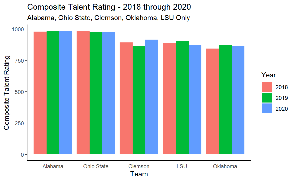
One thing I am interested in seeing is how “Talent Rating” has trended, over the three years that we pulled, for a select group of the top teams.
Let’s visualize it:
# Bar Chart displaying talent_rating for the teams
#   Alabama, Ohio State, Clemson, Oklahoma, and LSU for the years 2018 through 2020
team_talent_rankings_viz <- team_talent_df %>%
        filter(team %in% c('Alabama','Ohio State','Clemson', 'Oklahoma', 'LSU')) %>%
        ggplot(aes(x = fct_reorder(team, talent_rating, .desc = TRUE), y = talent_rating,
                    group = factor(year), fill = factor(year))) +
        geom_bar(stat='identity',position='dodge') +
      labs(x = 'Team',
           y = 'Composite Talent Rating',
           title = 'Composite Talent Rating - 2018 through 2020',
           subtitle = 'Alabama, Ohio State, Clemson, Oklahoma, LSU Only',
           legend = 'Year') +
      guides(fill=guide_legend(title='Year')) +
       theme_classic()

print(team_talent_rankings_viz)
Lastly, let’s write up some observations.
Conclusion
In this article I showed you how to test pulling data directly from an open-source API, write a function to do so more efficiently, explore, manipulate, and adjust data to fit your needs, and develop a clear and concise data visualization from that data.
The “Composite Talent Ratings” for the top teams should come as little surprise: Alabama is far and away the most talented team year in and year out, and we can see that this was the case for the three years we pulled. Ohio State is also a storied program and has had the talent to match up with Alabama the last three years, while Clemson, LSU, and Oklahoma, although certainly highly talented, see more variability year-to-year when it comes to their “Talent Ratings”.
There is plenty more you could do with this data, from correlating talent ratings with end-of-season outcomes or week-to-week win probabilities, to understanding how individual players contribute to this rating and if injuries could have major mid-season impacts, as well as many other potential data discoveries.
My hope is for you to use this introduction to dig into the data and explore further; please tweet me @JeffreyAsselin9 with your analyses or any questions, I would love to help out and cheer you on!
Thanks again to the maintainers of CollegeFootballData.com and RStudio. Happy Coding!
Distill is a publication format for scientific and technical writing, native to the web.
Learn more about using Distill at https://rstudio.github.io/distill.